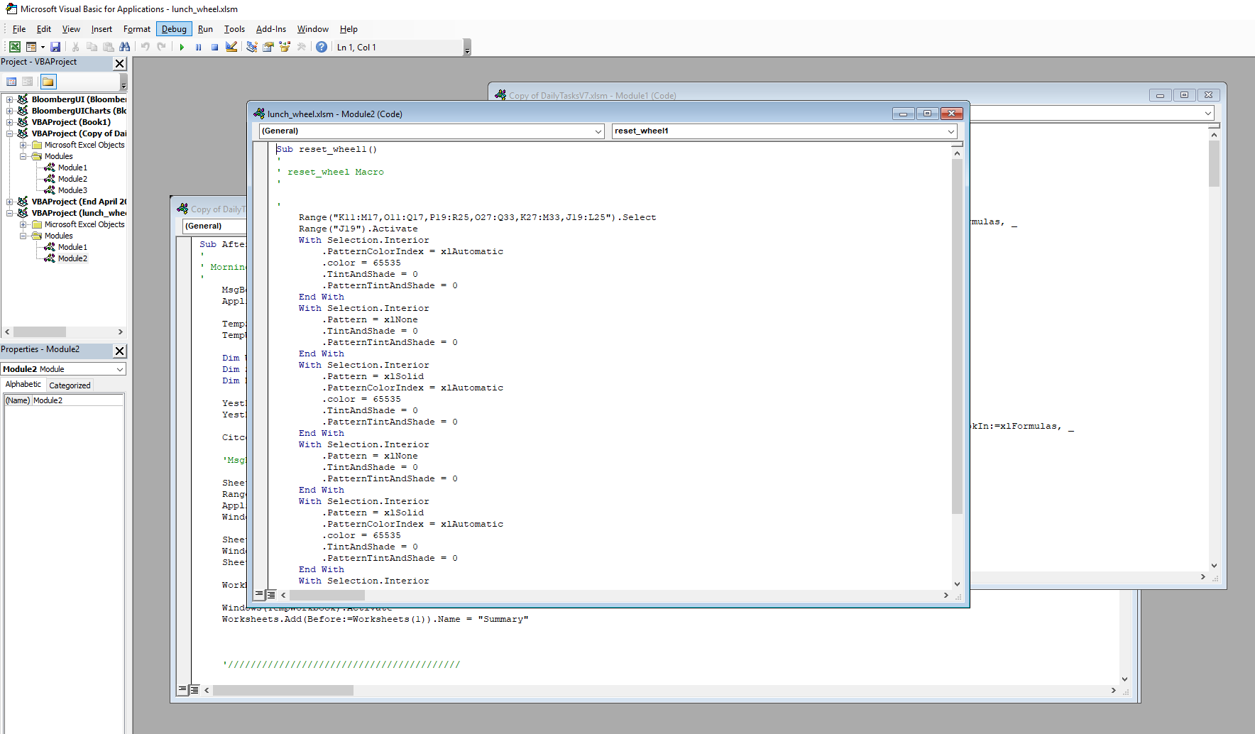
Excel VBA is a powerful tool which enables the automation of tasks in Excel. It can be used to automate many repetitive tasks along with more complex applications. This quick tip guide shows you how to open the Excel Visual Basic Editor (aka Excel VBA Editor) and get started with VBA programming in Excel. Having access to the VBA editor lets you write your own VBA code or … [Read more...]
Must have excel skills for Auditors
Introduction: We have earlier discussed in our posts the essential excel skill that are required to a general spreadsheet user so he can be more productive in his workplace. Today, we will discuss the skills and tools that are of great benefit for accounts especially those into the audit business. Our today's post will cover the following area relating to "most wanted … [Read more...]
Excel based Add-ins to Increase Your Productivity
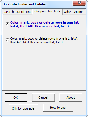
We will continue with our journey of finding excel add-in that boosts productivity of excel users. In our previous post we discussed excel add-in that are most popular among excel users. Since the list was complete, we will continue with the same topic in this post as well. Duplicate Finder and Delete add in: This is a very handy excel add-in designed to get rid of one of the … [Read more...]
The Best Excel Add Ins For Excel Users
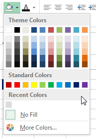
MS Excel's interface has been designed to increase productivity and ease of use. Despite these beneficial features, there are requirements that are not always met by the existing features of excel. These requirements are fulfilled by using VBA as we write macros and add custom menus or we can write excel add-ins. An Excel Add-in a set of code designed to do specific tasks that … [Read more...]
Performing Trend Analysis with MS Excel
Introduction: Excel has wealth of options to perform Trend Analysis. Trend Analysis is a very useful tool for business decision making and is a widely adopted procedure in Sales, Marketing, Finance, Operations and Inventory control. In today’s post, we will learn about options available to us to find the trend in our data and our focus will be mainly on quantities … [Read more...]