Often times when you execute a macro, the process isn't easily undone. You may have a macro that deletes certain information, or completely reformats your worksheet. In either case, you want to be sure that your workbook's users are absolutely certain that they are ready to execute the macro before running it. If the macro can be run by clicking on an object within the … [Read more...]
Hide/Unhide Columns
On occasion, you might find yourself creating a spreadsheet that has multiple columns all set up in a consistent format (i.e. quarterly sales figures for the past 5 years). As time goes on, you may add/remove data to the spreadsheet as needed. This may result in some columns not being used (i.e. in April only the first quarter's information will be filled out for the current … [Read more...]
Using a For Loop
"For" loop is used in a macro whenever you have an action that needs to be performed a set number of times. For example, if you want to change the fill color of the first 20 cells in a list, you could have the macro select the range and simply fill as desired. But what if you wanted to only fill the cells if they were blank, for example? Telling the macro to select the whole … [Read more...]
Automatically Create an Index for Your Excel File
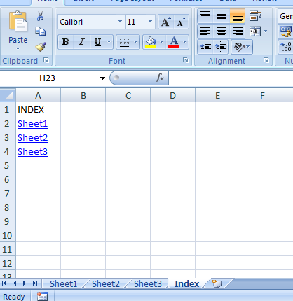
Do you want one central location where you can easily navigate to any worksheet in your file, and then navigate back with one click? This macro lets you quickly and easily create an index in Excel that lists all sheets in your workbook. The best part is that the index excel macro updates itself every time you select the index sheet! Indexing in Excel made simple. If you need … [Read more...]
Send Emails From Excel
Often times you'll find yourself working on a file in Excel that needs to be sent to a co-worker as an attachment. If you store your files on a shared network drive, it could take a little while to find your file, even if you know exactly where it is located. Even then, you may have to worry about attaching the wrong file if there are several saved with similar file … [Read more...]