Choosing between Vlookup and Index-Match formulas

Introduction

INDEX()+MATCH() and VLOOKUP(), both have their proponents and opponents. Both of these formulas perform almost the same function. Both have pros and cons. In today’s tutorial we will try to compare their usage and that how they can be used to get most out of them, when we should drop one and use another.

A comparison of syntax for the two formulas:

Index-Match are two different formulas combined to achieve the lookup task where as Vlookup is a standalone function from excel. Here is the comparison of the syntax of the two:

=INDEX(array, (MATCH(lookup_value, lookup_array, [match_type])), [column_num])
=VLOOKUP(lookup_value, table_array, col_index_num, [range_lookup])

Let’s start understanding them in context of some examples.

Comparison – 01: When you have to look on the right side of the table

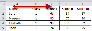
Assume the following case where we want to find the score against a name, this is a classic example of using VLOOKUP() function but we can also do it with INDEX()+MATCH() do as well. So lets compare the syntax we will be using:

There is not much difference in the length of two formulas as well as the arguments that they take. For Index we have four arguments because the MATCH() itself forms the second argument of the INDEX() function so both functions have equal arguments.

For this case, if you wan to look at right and have a shorter formula – go for VLOOKUP().

Case No. 02 – when you want to look at right of a Lookup column

This case is a little tricky for some of us. We are used to using VLOOKUP() to the right but actually VLOOKUP() can look at the left as well.

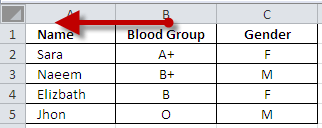
Referring to the Sheet 2 in the sample file, we have following table…

Now we have to look in the second column and fetch result from the first one. This one is very easy for INDEX+MATCH combination but what will be the case for VLOOKUP? Here is the solution:

With these two formulas, both can look to the left.

The first MATCH()+INDEX() formula just move the lookup range to the left side giving the required result. But the VLOOKUP() formula here is tricky. This formula create an array where the values of second column comes first and the first column comes second – thanks to CHOOSE() function. When we look at Evaluate Formula tool bar it looks like:

=VLOOKUP(C7,CHOOSE({1,2},B2:B5,A2:A5),2,0)
=VLOOKUP(“O”,CHOOSE({1,2},B2:B5,A2:A5),2,0)
=VLOOKUP(“O”,{“A+”,”Sara”;”B+”,”Naeem”;”B”,”Elizbath”;”O”,”Jhon”} ,2,0)
=Jhon

Hence if a user is comfortable with using an array formula (with Ctrl + Shift + Enter) he can use VLOOKUP() function to look at left as well. For the case of length, MATCH()+INDEX() is still smaller then its VLOOKUP() counterpart hence for this part we will recommend MATCH()+INDEX().

Case No. 03 – when you want to have variable column offset by matching a criteria

It is not unusual that a user may want to set the column offset in VLOOKUP() by matching some criteria. This eliminates the task of looking up at the table and entering the column offset value manually. In this third case, we will check both the function for the ease with which we can set this column offset criteria.

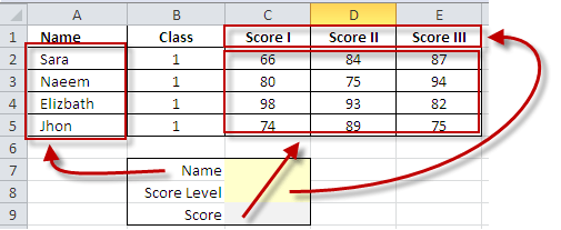
Again referring to the Sheet 3 in the sample workbook, we are interested in setting a cell as a container for Scores (Score I, Score II,).

Here score level is our criteria. Let’s see how we can achieve it with these two formulas:

Here we have used the reference form of INDEX() function that is similar to its working with OFFSET() formula. For such a construction, we first point a reference to the entire table and then uses MATCH() function to tell INDEX() the column and the row numbers. this approach to solve the problem uses seven arguments and is 53 characters long.

The second method was to use the VLOOKUP() function but it is to be noted that VLOOKUP() again relied on MATCH() function to set offset column. This time, the second construction is smaller then MATCH() construction and is comparatively simpler. Hence for this case the winner is VLOOKUP()!

Case No. 04 – Looking Horizontally

For this case, INDEX()-MATCH() is a winner without even going for comparison with VLOOKUP(). VLOOKUP() stands for vertical lookup and for looking into row, we have its counterpart HLOOKUP() to do the task.

Conclusion

We finally conclude that both the formulas are useful for a user. If a user has a table with lookup range on the left that the ultimate choice should be VLOOKUP() as this is the easiest one to go with. But if the lookup range is on the right and we have to fetch the data from left or if we want to look in a row for certain value then we can opt for MATCH()+INDEX(). If we want to look in row then we have either to use INDEX()+MATCH () or will have to revert to HLOOKUP.

Please download the workbook to see the examples mentioned in this tutorial. Thank you