Add Values Between Two Dates

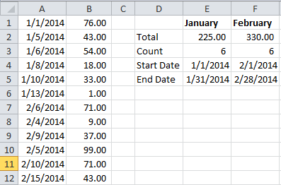
If you are keeping records in an Excel spreadsheet that contains a column for dates and another column for some figure that can be added up, such as sales, you can easily use a formula to add values between two dates.

The formula uses the

equation, which basically adds up a range of cells based on a certain set (or sets) of criteria. In this case we will use two dates as the start and end point to tell the formula to add up any values that are found in between those dates.

Add Values Between Two Dates

In the image above, there are dates in column A, and a list of number we want to add in column B.

You can see that there is also a little table in columns D:F that show the end result. Here’s how you can get there.

In cell E2 (the January total), you would enter in the following formula:

=SUMIFS($B$1:$B$12,$A$1:$A$12,">="&E$4,$A$1:$A$12,"<="&E$5)

You can then drag that formula over to cell F2 (or however far across you need it to go) to get totals for other months.

Step-by-step, here is what that formula is doing:

• $B$1:$B$12 – Defines the range of cells to be added if they meet the criteria to be defined later in the equation.
• $A$1:$A$12 – Defines the range of cells that the first criteria should apply to. In this case it is the range of dates.
• “>=”&E$4 – Defines the “start date”, which in the example above is entered into cell E4. However, if you wanted to enter the start date directly into the formula, you could replace “>=”&E$4 with “>=1/1/2014”, or whatever your start date is.
• $A$1:$A$12 – Defines the range of cells that the second criteria should apply to. In this case it is the same range that the first criteria should apply to. You could define a different range if you needed to.
• “<=”&E$5 – Defines the “end date”, which in the example above is entered into cell E5. Just like the start date, you could enter “<=1/31/2014” directly into the equation if you wanted to.

A couple things to point out about this equation:

• The range of dates do not need to be in any particular order. Notice in the example how the January dates are all sequential, but the February dates are out of order. The formula would have produced the same results if the list was sorted by column B, or if it was in no particular order whatsoever.
• The
  You must be logged in and have an active membership to view this content. Please register or login to continue.
  will not work in a Excel 97-2003 workbook. Instead, you can use the
  You must be logged in and have an active membership to view this content. Please register or login to continue.
  equation to achieve the same results.
  • =SUMPRODUCT(($A$1:$A$12>=E$4)*($A$1:$A$12<=E$5),$B$1:$B$12)
• Notice the count row under the total row? This is achieved by using the
  You must be logged in and have an active membership to view this content. Please register or login to continue.
  formula, which is very similar to
  You must be logged in and have an active membership to view this content. Please register or login to continue.
  , except that it counts the number of cells that meet certain criteria rather than sum up a range of corresponding cells. This could be a useful addition to the spreadsheet if, for example, you wanted to get an average sale amount.
  • =COUNTIFS($A$1:$A$12,">="&E$4,$A$1:$A$12,"<="&E$5) – This basically looks at the dates in A1:A12 and counts them if they fall in the range of dates given in E4 and E5.
• You can easily change the dates that get added by changing the values in E4 and E5 (and F4:F5). This will let you  add up all the amounts on the same day, during a week, month, year, or whatever time period you choose. 

What applications would you use this sort of formula for?