Recently, I was working on a budget for a class that I was putting together. Most of the expenses that would be incurred were fairly straightforward and would increase in proportion to the number of students that were in the class. For example, student manuals cost $11 per student. Easy enough to find out the total student manual cost by multiplying by the number of students, so no problem there.
However there was one expense that really did not correlate exactly to the number of students. This expense was shipping costs.
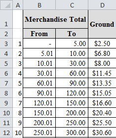
The supplier that provides the student manuals charges shipping costs based on a rate table where any orders whose total cost is between two amounts gets charged a certain rate.
The issue for me is that I wanted my budget to automatically update when I entered a new number of students. Looking at the table above, and assuming an $11 per student cost, I would be paying the $8 rate for shipping whether I had 1 ($11) or 2 ($22) students in the class. If I had 3 ($33), 4 ($44), or 5 ($55) students I’d be paying the $11.45 rate.
The VLOOKUP formula seemed like it would be the logical choice for this sort of problem, but the issue with VLOOKUP is that it doesn’t know how to define an upper or lower limit to the range.
To use the VLOOKUP price ranges formula, I needed to also use a couple other functions like SUMPRODUCT, and ROW.
My Excel Workbook is set up with tabs for each individual course, and another tab with the shipping cost table shown above.
- Shipping Worksheet B3:B35: Merchandise totals “From” column.
- Shipping Worksheet C3:C35: Merchandise totals “To” column.
- Shipping Worksheet A3:D35: VLOOKUP range.
- Class Budget Worksheet E6: Total cost of merchandise for that class.
With that information I got the following formula:
Here’s a breakdown of what is happening in this formula:
- VLOOKUP: This is using the range A3:D35 to look up the correct shipping cost. Column A was populated with sequential numbers to make the VLOOKUP easier. There are other ways to look this information up, I just chose this way for now.
- SUMPRODUCT(–(Shipping!B3:B35<=E6)*(Shipping!C3:C35>=E6)): This takes the ranges of B3: B35 and C3:C35 to find the set of high and low merchandise totals to find the pair that contain the value in cell E6.
- ROW(Shipping!B3:B35): This gives the row numbers 3 to 35. When combined with the SUMPRODUCT part of the formula, this will tell you the row number corresponding to the high and low totals that contain the value we are concerned with. Combining this with SUMPRODUCT provides the VLOOKUP with the look up value it needs.
- -2: There are two header rows so we need to subtract them from the result so the VLOOKUP will find the correct number in the table.
