Introduction:
“Comments” or “Annotations” add a lot of value to data. They are frequently added by programmers to their codes to make them more understandable. Adding appropriate comments to a program or document is a good practice because a programmer or writer might forget, over time, the purpose of the code. For someone who was not part of the project it could be really difficult to grasp the theme of the code (or document).
The same rule is applicable to the reports we create in MS Excel. For longer and more complicated sheets, we regularly add comments to cells to provide further context.
In this tutorial we will see how we can annotate a pivot table. You can download the companion worksheet from this link.
Adding Comments to a Cell:
Adding comments to a cell is simple. Select the cell and simply:
- Press Shift+F2, this will insert a comment to a cell.
- Use Key Tips feature – you can press Alt+R+C to a comment to a cell.
- Or alternatively you can point your cursor to Review Tab and select add a comment.
Comments are shown in excel by a small red triangle (flag) on the top right side of a cell. For convenience, excel has the option to show or hide all the comments that is accessible through Review>Show All Comments or Hide All Comments.
Adding Comments inside a Pivot Table:
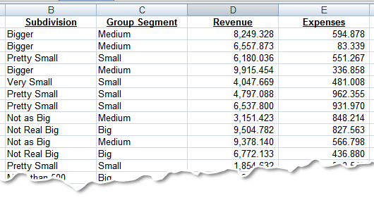
Consider the list of data as shown in following picture. It has four fields (heading): Subdivision, Group Segment, Revenue and the Expenses. We will create a pivot table from this to analyse the data.
The resulting pivot table has the following layout. The pivot table clearly explains how the data is distributed for various subdivision, group segments and their respective expenses and revenues.
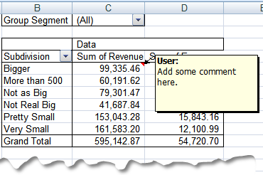
Lets take up an example – we want to add a comment to Subdivision: Bigger and Revenue Value of 99335.46. We can do it by simply pressing Shift+F2 – a way we used to comment on a normal, non-pivot table cell. Following in this manner we can add additional comments inside of cells.
In order to view or hide all or some of the comments, we can use Show or Hide All Comments:

Till this point everything is OK – we have our comments placed inside the correct cell. The problem starts when we try to filter the pivot for some criteria for analysis.
Managing comments with a changing pivot table:
As we change the criteria from the Pivot Filter – the following situation occurs:
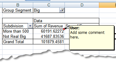
Let’s make use of the filter in the pivot table. The pivot table is updated for the selection segment “Big.” As the entire table is updated, we are faced with the problem we have already pointed out in this article. It is clear that the comment that we added to a different cell is still there – we meant this comment for revenue for ”bigger” subdivision but this is now showing against “More than 500.” This shows us the obvious limitation of comments placed inside of pivot tables.
The WorkAround # 1:
The workaround in this case is to add a column in the original pivot table with comments. In the following screen shot we can see the fifth field added to our data that contains the comments. The final list looks like the below one:

When we create a pivot table, we will not be able to see these comments but they are visible when we double click on any value in the pivot table, as double clicking the value will open that specific entry in to a new worksheet. When you double click the following entries are displayed (clicking 99335.46168)
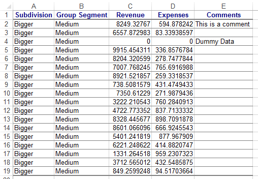
You can see that the comments are visible against each entry.
WorkAround # 2:
The second workaround is yet another trick. As we know that pivot tables are really good at summarizing data, we will create a pivot that has all the information it can hold. There is a limitation when it comes to large pivot tables – but it should be remember that for large pivots, we often do not use all of the fields available to use, but just few of them to create scenarios.
So in this case we have four fields only. That can be arranged by removing Group Segment from Report filter and bringing it to Row Labels (above subdivision). This gives us the following pivot table.
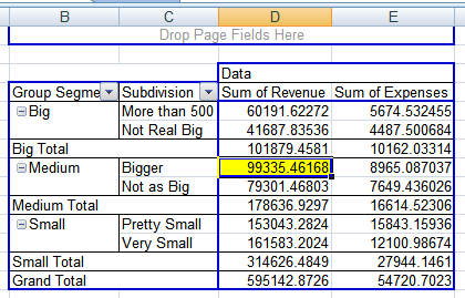
With this, we have eliminated the need for a filter and hence the event where comments are mis-located. We have all the required information in just one pivot table – feel free to comment over it.
Additional Annotation:
The above table is not symmetrical. By symmetrical we mean that there are no values of Revenues and Expenses for the Group Segment Big, Subdivision Bigger and Very Small or Pretty Small. Similarly no such entries for More than 500 and Pretty Small for Medium segment group. That is making this table unsymmetrical.
In order to improve its looks and make it more professional, we can add some dummy entries to the original data like below:
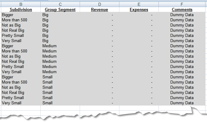
The above arrangement will result in the following Pivot table update: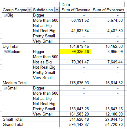
As we can see that most of the options are availed and we have also listed for all the options we could have needed, we can now easily comment on this pivot table with conventional comments.
Conclusion:
Though the options for annotations are limited, there are workarounds. We have seen two of these workarounds by adding a comment column to the original worksheet and the second one by adding all desirable variables such that there is no need for filtering the pivot – this might not be the ideal solution it works, nevertheless.
Please download the file from this link to see a live version of the above examples.