Whenever you are dealing with lists it seems like you always are looking to count how many of a certain item is in the list. Maybe you want to count how many cars were sold by a certain salesperson, or how many times an employee called out sick. Luckily Excel makes it easy to count cells meeting certain criteria just like this.
Count cells meeting certain criteria with Excel’s COUNTIF function
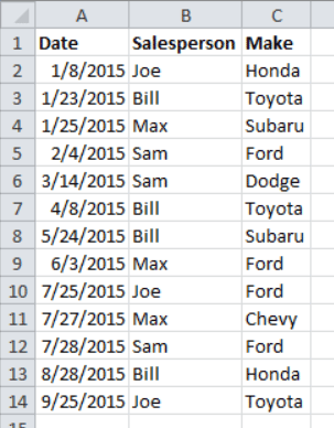
 Let’s say we have a list of dates that cars were sold on a used car lot, the salesperson who sold the car, and the make of the car. This list is great information, but we want to know who sold the most cars. You can see the screenshot of this list to the left.
Using Excel’s COUNTIF function we can count cells meeting certain criteria to figure out who sold the most.
To make our lives easier, let’s put a list of the names of each member of the sales team either off to the side of this sales list or on another sheet. Joe, Bill, Max, and Sam. In my sheet I have this list in cells E2:E5.
In cell F1, I have the following formula:
=COUNTIF($B$2:$B$14,E2)
This formula takes the range B2:B14 where we have the names of the salespeople who sold the cars, and counts how many times they appear in that range. E2 contains a salesperson’s name, so it uses that cell as the criteria to match against. We could have just as easily typed in the salesperson’s name in place of E2 in the formula, but since we have several names to look up we can use the cell reference to avoid having to re-type the formula.
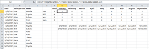
Next, copy the formula down to fill in next to the remaining salespeople to get the results. If you need to visualize this, check out the screenshot at the end of this article.
The results based on the list in the screenshot are Joe: 3, Bill : 4, Max: 3, Sam: 3.
This is great, but looking at the list it seems like Bill stopped selling as many cars after May. What gives Bill?
Count cells meeting multiple criteria with Excel’s COUNTIFS Function
What if we wanted to find out who sold the most cars in a certain time period? We can use Excel’s COUNTIFS function to count cells meeting multiple criteria.
I want to find out who sold the most cars each month, but the same concept we’re using could apply for any time period – weekly, quarterly, annually, or any other custom time period you would need to look up.
Continuing from the earlier example, let’s add columns for each month next to the total we set up in column F. So, column G would be January, H would be February, etc.
Now, since Excel refers to dates using a number rather than the normal month/day/year format we might be accustomed to we have to enter the range of dates we are interested in looking at. This may not be an ideal solution, but it does allow for custom date ranges.
Below our table of salespeople and months let’s add the first day of the month and the last day of the month so we can use those dates in our formula. In my sheet, I entered the first day of the month in row 7 of the month’s column, and the last day below it in row 8.
In cell G2, which on my spreadsheet is the cell that will display Joe’s sales tally for January, enter the following formula:
=COUNTIFS($A$2:$A$14,">="&G$7,$A$2:$A$14,"<="&G$8,$B$2:$B$14,$E2)
This formula is similar to the COUNTIF formula we used earlier, except COUNTIFS allows you to specify multiple criteria to fine tune the results.
You will also want to copy and paste this formula down to the other salespeople, and across to fill in for the other months.
We’ll break this formula down to each set of individual criterion.
$A$2:$A$14,”>=”&G$7
This looks at cells A2:A14 where our dates are and wants to find any that are greater or equal to cell G7, where I have the first day of the month listed.
Note that the date used in G7 is simply the start date of the time period we’re interested in. It doesn’t have to be the first day of a month, although in this example it is. It could be the first day of the quarter, week, or some other custom time period. Same idea applies to the last day of the month. Use whatever beginning and ending dates that make sense for your situation.
$A$2:$A$14,”<=”&G$8
This basically uses the same logic as the previous criterion, except it is looking for any dates that are less than or equal to the last day of the month, which are in cell G8.
$B$2:$B$14,$E2
Finally we use the same logic that we used in the previous COUNTIF formula to limit the results to only one salesperson. Cells B2:B14 contain the salesperson’s name who sold a car, while E2 contain the salesperson that we’re looking up.
Putting all that logic together in plain English, we’re asking COUNTIFS to count any cells where the date is greater than or equal to the first day of the month and less than or equal the last day of the month, and where the salesperson is the one at the beginning of the row.

If we wanted to also find out who sold the most of a certain make of car, we could add the condition $C$2:$C$14,”Honda”. This would show all the Hondas sold by a particular salesperson in a given month.