Introduction:
Though there many “dedicated” application available for project managers to manage their projects, like MS Project or Primavera Project Planner, we can also create a project time line in MS Excel! In today’s tutorial, we will be exploring the ways to create a project time line in excel, along with the terminology and some theoretical background of project management.
So, what is Project Management?
A project can be defined as an activity targeted to achieve a preset target with marked limitation within a given time frame and cost budget. Managing a budget is critical as the resources are scarce – time, people, financial resource. A little delay can lead to problem or even project failure. Hence a project management tools is highly desirable.
What is work break down structure in project?
The project activities can be broken down into smaller step or set of activities that will eventually execute the project. A work breakdown structure makes it easy for manage to complete the project. It shows the precedence of activities in a project.
What is a Milestone in a project?
A milestone marks the completion of an activity in a project. As we have crated work units in work breakdown structure, their completion is marked with a Milestone in project. Let’s take up an example and see how we can produce a project time line:
Example:
Consider a family that is planning to construct their home. They consult a Civil Engineer that gives them following action plan to build their home:
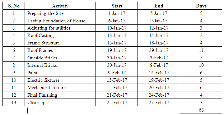
In the above chart, there are some activities that are dependent on others and some will start at the same time.
Let’s setup a sheet and see how we can produce a timeline. As a starting point we must remember that project timeline has activities on the left hand side and the time on the top horizontal axis.
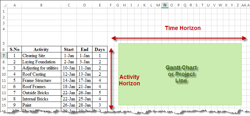
On the time horizon we will mark each cell with a date and then fill the color accordingly to make a Gantt chart or project line effect. On the project sheet will mark a start date and then the time horizon will move day by day as in the following picture:
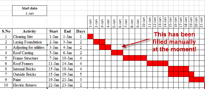
This has been done by manually filling the cells to create a project line. But we will be discussing a formula that will take start and the end dates and will do the needful.
The formula for filling up the cells:
As we know that there is no formula that can fill the cells with a color, we have to take help of conditional formatting. The conditional formatting will work on the logic that if the cell contains certain value, the cell will be filled by the color and vice versa.
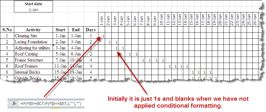
So let’s assume that cells with value of 1 will be highlighted and anything else will not be. Let’s create a formula that will fill the chart with 1s for date ranges.
The formula:
The formula that we will be using is:
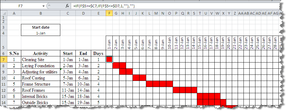
=IF(F$5>=$C7,IF(F$5<=$D7,1,""),"")
…is present in the cell F7 of the sheet Gantt chart.
Understanding formula:
The formula works by comparing the start date that is present in C7 for being greater than or equal to F5 that is a date on the time line. The formula still goes on and tests the second criteria that if the end date is less than the date in the D7. This makes sure that we only get 1 in the cells that are within the date bracket of the activity. Everything else will have a blank space in the cell.
Now let’s understand the cell referencing in the formula.
- The dollar sign in F$5 means that when we move formula downward, the cell will still refer to the time line date by not changing the cell reference. However the cell reference will change when we move it rightwards.
- The dollar sign in $C7 makes sure the when we drag the formula right ward, the formula still refers to the start date that is present in column C7 but he reference may change when we move it downward.
- The dollar sign in $D7 does the same function as that of $C7.
Understanding Conditional Formatting:
The initial step is to:
- Select the cell F7.
- Go to Conditional formatting menu: Conditional Formatting > Manage Rule > New Rule > Use a formula to determine which cell to format. This will lead you to following menu with following space for a formula:

- In this space we will write the condition that where ever there is 1 it should be formatted (color filled etc) and rest should be left as it is. Here is the formula.

The default format when you select the cell is $F$7 but we need to make reference relative so we will remove dollar sign from it.
- In the same dialogue box where we have entered the criteria for highlighting cells, we have a tab to format the text, as shown in the following picture.

From this dialogue box we will format cell to be:
- Filled with red color
- The font color should also be red so that 1s are not visible.
- Once done, press ok to close the format dialogue box, press apply to apply it to the selected range and again press OK to close the conditional formatting dialogue box. The final result should look like this:
Conclusion:
This has created a simple project line also called Gantt chart for project management. Please download file from this link and see how formulas in the sheet actually work.


