Creating a Project Timeline in Excel
A project is a onetime activity that can span over varying length of time. A project could be an activity that can finish in a day or it could cover months and years. Project management is the process of managing this activity. As the complexity of the project increases, it becomes more and more difficult to manage it, hence require more and more skilled people. However, whatever be the project and however is handling it, one tool is always there to help them – that is called Gantt chart or simply the project timeline.
In this post, we will discuss methods that can be used to have a project time line in Excel. The question might be asked why to use excel when there are specialized software available for project time lines. The answer is simple, the cost of such software some time way more than one can afforded for minor projects. Or even if the software and less expensive, it might have a steep learning curve. Hence people revert to the use of MS Excel for project management.
How does a project time line look?
Most of the project time lines or Gantt charts have activities on the right hand side and the date line on the top of the table. This makes it easier to list down all the activities one by one. Using, the activities are sub divided into smaller activities and still smaller activities – this is called the Work breakdown Structure of a project.
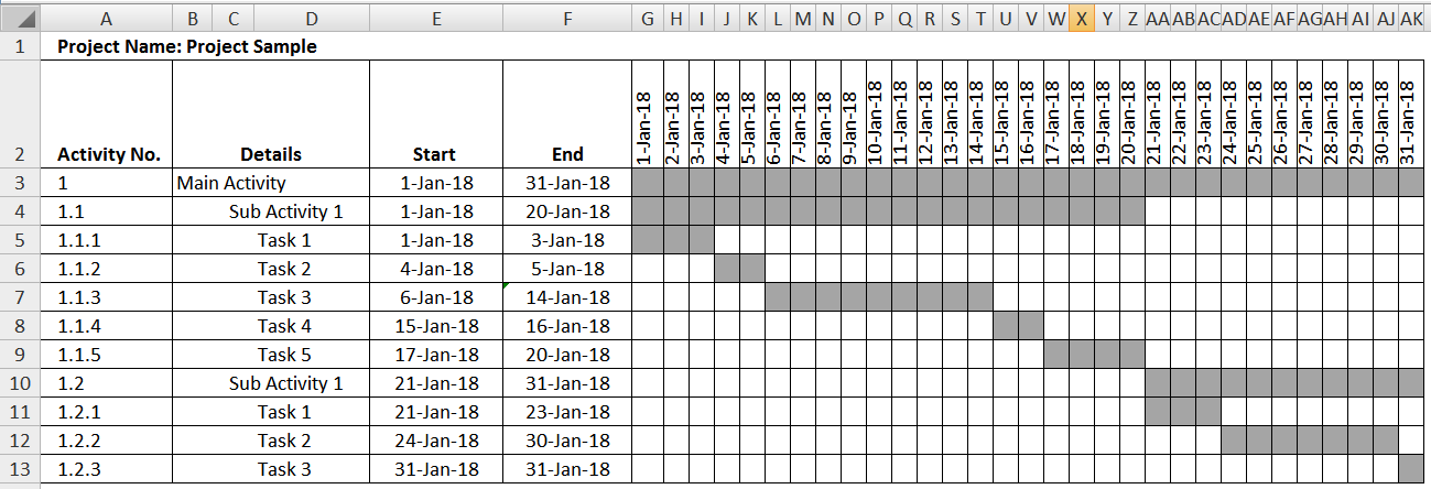
The Gantt chart uses indentation to mark sub activities. Sometimes number separated by a decimal place is used to show the hierarchy. The activities column is followed by two more columns that describe start and the end date of the activity. Here is a sample of how does a Gantt chart look like.

Creating your own project time line:
Various website offer ready to use templates for project time line, but we can also create our own as per our personal requirements. In the following lines, we will understand how to create the above project line.
Step 1 – Work Breakdown Structure
Make sure you have one! Without WBS, it is difficult to plan a Gantt chart, if not available, you can create some dummy activities just to fill the space. It will make it easier to understand the flow of the process. You can use either indentation for creating hierarchy of activities or use consecutive column to put in different activities.
In our case, we have used different column to put in the sub activities.
Step – 2 Have a Stand and End Date Column
The start and the end date describes the start and end date for all the levels of the activity. The start and end date for main activity should encompass all sub activities and tasks. There two possibilities to create end date and start date in Gantt chart:
- Put start and end date manually.
- Put start date and enter number of days required for that activity to complete. The end date can be obtained by adding the number of such day.
End Date = Start Date + Days Required To Finish the Job
In our case, we have entered the values manually.
Step – 3 Creating Header Row with Dates:
This is amongst the most important part of creating a project time line, because without dates, it will not give us our desired result. We start with a date and then keeping adding one to it so that it progresses automatically.
Thus in G2, we put the first date manually, and from it onward to the right, the date is calculated by adding one to the proceeding one. G3 becomes G2+1, G4 = G3+1 and so on.
Step – 4 Showing the activity with shaded area.
One done with these three steps, the next and the most critical step is show the activity progress by shading some cells. For smaller projects with less frequent steps, we can do this task manually. But in case you want your activities progress to be date dependent then will require some excel understanding.
In order to make progress date dependent, we will make use of conditional formatting menu.

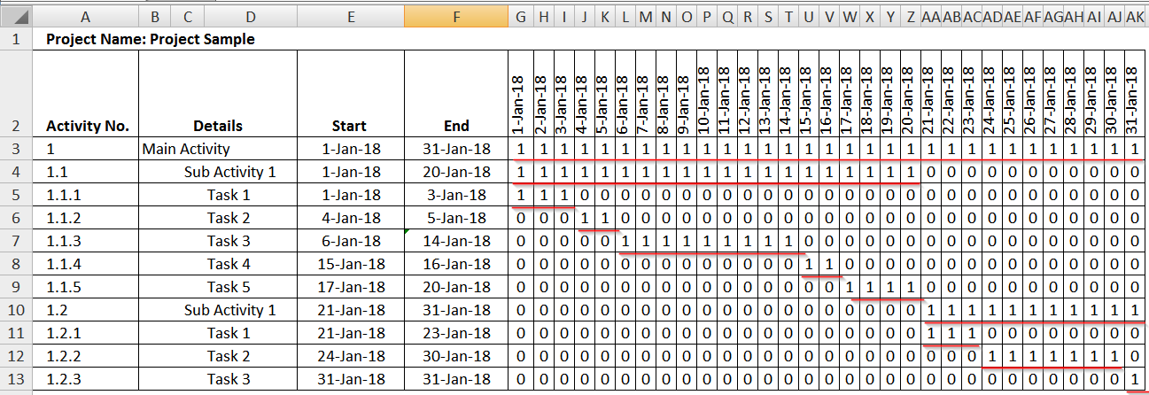
We use and IF() function with AND() to get our desired result. The formula works by evaluating the AND() function. This function checks if the date in the header row lies in date bracket of start and end date. If it lies, the formula will return 1 and else will give 0.

For example taking up the first cell, in G3, the formula is evaluated in the following manner.
=IF(AND(G$2>=$E3,G$2<=$F3),1,””)
The first part to be evaluated in G$2>=$E3, G2 is in the header column, this compared the time line value in cell G2 with start date in E3, we have fixed row referencing style for G2 and fixed column refereeing style for E3, as we will be dragging the formula, rightwards and downwards.
The second part of the formula G$2<=$F3 will compare if the time line value is less than the end date. If yes then AND() will return a TRUE, the formula only works when we have both TRUE. The result will be a table with 1 and 0.
You can see he progress in form of arrays of 1 in rows.
Step – 5 Applying Conditional Formatting
Now we will use these 1s and 0s for conditionally formatting cells.
- Select the entire range from G3:AK13.
- Go to Conditional Formatting Dialogue Box and select Rule Manager.
- From there select New Rule. This will make a new rule.
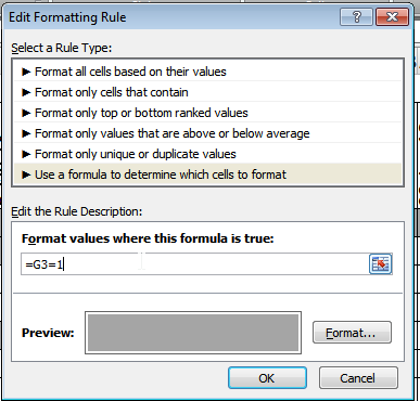
- Using New Rule, select the last options from dialogue box that sets criteria for cells to be formatted based on cell value.
- Select formatting from same dialogue box – select a color to fill and the same color for font in the cells.
- Remove fixed cell referencing from the formula section.

- The formula should be =G3=1 that means that when applied it will have all the cells that are equal to 1.
- Press Ok to exist the dialogue box, press on one again and press Apply to apply the formatting.
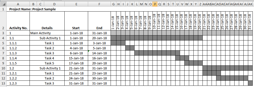
Once done the final output should look like.

Conclusion:
You can see that cell, with value 1 are only filled with color creating the project time line effect. The entire cell there had zero are now blank. In this ways we can create the project timeline in excel. Please download this file to see how things works and create your own time line