Exploring Excel’s Internal Audit for Formulas

Introduction

Formulas are very common element of a spreadsheet. Smaller sheets tend to have relatively small number of formulas where larger sheets may span over many worksheets. The formulas in such large sheets are not easy to understand. With Excel’s Internal Audit for formulas,  we have a convenient way to do internal audit for formulas and for a tool that can make audit formulas easier.

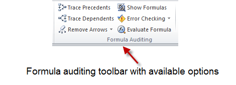
MS Excel has a built in formula audit toolbar that can be used for the purpose. To access this toolbar, one need to switch to Formula Tab > Formula Auditing and we can use the options available to cross check the formulas.

Every formula has usually two parts:

1. Input variables (or simply input cells)
2. Output variables (or output cells)

And error can be caused by numerous reasons in the formulas, some of them are:

1. When input variable leads to a wrong cell
2. When input’s input lead to a wrong cell
3. When output variable is feed to a wrong cell

And so on.

So let’s see what options are available for a user to trace such errors

Tracing errors from Inputs –tracing precedents:

Precedents are input to a formula as the figure shows its label. When we select a cell with formula and press the button, all the cell that are related as input to a cell are displayed through a blue connector. This connector has an arrow on the side that points to cell with formula and a filled circle on the other that resides on the input cell.

Let’s take up the example sheet we can see that:

The cell E1 is the cell with formula, and the input comes from the range A1:B1. The direction of arrow explains that cells that are input and the one that are output.

We can still trace it further, if the input cell also has precedents. For example in the following screen shot, pressing the trace precedents button twice will show the input’s input cells – but with  distinction of light and thick yellow lines:

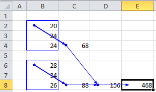
We can see the light and dark lines to distinguish direct and indirect inputs to a cell’s formulas. And this is just not twice that you can press the button, you can press it multiple times to further trace the formula as shown in the following picture:

Tracing errors from Outputs –tracing Dependents:

Tracing dependents is the same as that were precedents – you just need to press it times you want. Here it is not required for a cell to have formula instead a cell should be connected to a formula to have dependent cells.

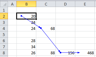
For example in the above picture, the cell B2 act as an input to C4, that acts as input to D8 and that acts as input to E8. Again the direction of flow is made clear by using circle and arrow head on the line.

Tracing errors from Outputs –tracing Dependents:

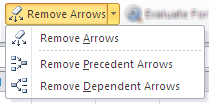
When we are done with tracing formulas, we can remove arrow from the sheet. This is done by using Remove arrow button. This allow us to remove either precedents or depends or both of them, thus returning sheets to its original state.

Showing formula with “Show Formula” Button:

Another way to trace error is to visually inspect the formula under consideration. This allow us to see for error like:

1. Referencing problems : problems caused by wrong use of fixed and relative referencing
2. Multiplication / Division by wrong number
3. Even wrong references to cell can be traced.

When we use this tool, the output of the calculated figure in a cell is replaced by the formula:

Another example can be seen from the following situation, where the fixed referencing style for cell B2 is missing that will cause the value error and wrong multiplication of cells:

Using “Error Checking” button to find error:

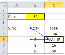
If you are not sure whether if there is an error or not in the sheet, you can use this button to trace automatically an error. As you press this button, the cell with error will automatically be spotted and with precedents that are causing error.

For example in this picture, there are multiple formulas, but only cell that has error has been highlighted and its precedents are being show:

Using evaluate formula button:

This is perhaps the most used and the most useful of the options that are available for checking errors in the formulas. With this option we can evaluate the formula step by step and see the results if they are coming as supposed to be.

The formula evaluates option follows traditional rules to evaluate the formula:

1. Expressions between parentheses (brackets) are given preference and are evaluated first.
2. This is followed by multiplication and division.
3. This is followed by addition and subtraction.

In excel formulas; curly brackets donate array formulas, so we have only small but multiple brackets to write an expression. For example in the following formula:

=((2+3)*2+(6/2)+1)

The formula will be evaluated as follow:

1. Brackets first:
   1. 2+3 will be 5
   2. 6/2 will be 3
2. Result expression (5*2+3+1) will be done like
   1. Multiplication first – 5*2 will be 10
   2. 10+3+1 will be 14
3. The final result will be 14.

Now let’s see how this formula is evaluated by the “Evaluate formula” option:

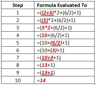
In this way one can see if the formula (particularly the precedence of operations) is working correctly.

Going Beyond formula auditing toolbar:

Using formula auditing tools bar is at best a correct approach to checking errors. This is because here you are checking for “existing” error and this a corrective approach for eliminating errors.

A better way is to use preventive approach to avoid errors. This approach includes some of the following options:

1. Using modular design of spread sheets
2. Using smaller – multiple formulas rather then one single-large formula
3. Using Tables instead of simple ranges
4. Using named ranges
5. Documenting your work as your proceed with design of spread sheet.

A modular design is a design that divides a (spreadsheet based) model into small parts. This simplifies the overall structure of the worksheet and we can check individual components for the error – one by one, if there is one.

Using smaller and multiple formulas do the same thing. Try evaluating a large formula in the evaluate formula window and you will realize how difficult it is to follow up with it.

The use of table will allow your formulas to be updated automatically if the data is appended in the table, without need for manually doing the same task. The named ranges do the same work.

Documenting your work will make it easier for yourself and for anyone that works with or troubleshoot your spreadsheet.

In this way you can prevent error from the start.

Conclusion:

In this article, we have used the tools available for auditing the formulas in a spreadsheet. There are multiple options available at our disposal but the best approach is to avoid adding error to our sheets. Please download this file to for the tutorial.