A how-to guide to conditional formatting based on another cell

Introduction

The conditional formatting is used for highlighting cells that meet certain criteria. These cells can be duplicate values or they may fall within certain limits or a similar criteria. In today’s tutorial we will be explaining how to highlight a cell’s value when it meets criteria in a cell.

Most often we use cell referencing to set criteria for conditional formatting when we know that the criteria will change hence in this post we will show how to setup conditional formatting for such cases.

Here are examples to explain the functioning:

Highlighting First Names with Conditional Formatting:

Let’s assume that we have a list of names (first and second name) and we want to highlight all the names that have certain first name.  The criteria cell for this case is B3 that contains the first name we are looking for, whereas the list is located in $A$3:$A$10. The excel sheet looks like following:

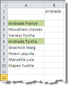
The question is how to setup a formula where i can highlight the names with first name – “Andrade”?

Our formula:

Following picture shows the formula that serves the purpose:

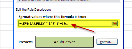
The formula actually works by finding the space between the first and the second name and then taking up the first name and ignoring the second one. This does not finish the formula, in order to return true or false the result need to be compared with value in $B$1 and the result will either highlight or not highlight the list. Here is step by step solution of the formula:

1. We start with the formula =LEFT($A3,FIND(” “,$A3)-1)=$B$1 and start evaluating the expression from inside out.
2. The first expression evaluated is $A3 that represents the name in the list – Andrade France.
3. The second expression evaluated is FIND(” “,$A3) that is evaluated when the function looks for the space in text in cell $A3. This evaluates to 8 for this case as space character is the eighth character in the text. The final expression thus becomes =LEFT(Andrade France, 8-1)=$B$1.
4. In the next step, one is subtracted from 8 giving us the exact length of the first name.
5. Now the first name is extracted using the LEFT() function that starts from the left side of the text and extracts 8 characters that forms the first name.
6. As a last step, the extracted name is compared with the criteria value and TRUE or FALSE is returned.

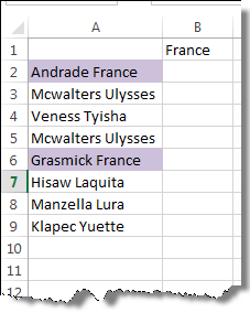
After setting up this formula, we will set the formatting style for to for conditional formatting and we have out highlighted list of names.

Highlighting second name with conditional formatting

Just like what we did for the first name, we can also setup a formula to search for and highlight the second name in a list. (Or simply anything that follows after the first space in a sentence). For example, for the name “Andrade France” the second name is “France” that can be highlighted in a list. The formula used in this case will be:

=RIGHT(A2,LEN(A2)-FIND(" ",A2))=$B$1

Steps:

The formula will evaluate in the following steps:

1. The first thing to evaluate is A2, the first argument of the RIGHT function that will evaluate to Andrade France.
2. The next expression evaluated will be the function LEN() that will be evaluated to 14.
3. This will be followed by evaluation of FIND() function that will find the space in the text – again it will be the eighth character in the text.
4. The difference of the LEN() and FIND() will give use the length of the second name. For this case it is 14-8 =6.
5. In the second last step, the RIGHT() function will extract the 6 characters from the right side.
6. Lastly the name will be compared with the criteria to return a TRUE or FALSE as result.

We can set the conditional formatting to highlight the second name as well in the text.

Highlight  values in a Range:

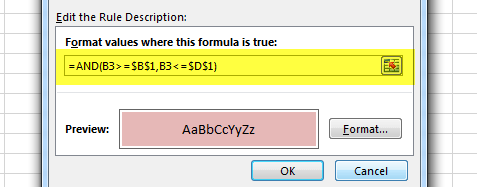
Another example could be to highlight cell based on range of value. We can also do it using the conventional (and somewhat more easy method of using menus) method. But in this section we will try to learn an new method that will make use of a formula AND() to explain the process. The following is the screenshot of the formula:

Steps:

Here is how the formula is implemented:

1. The formula works by using the logical function AND().
2. Within this function there are two conditions that need to be fulfilled to get a TRUE. Once get true the conditional formatting will be triggered and we have cells filled with color.
3. The first argument makes sure that value in the cell is greater than or equal to the criteria value by comparing the two – B3>=$B$1, here B3 is the cell in the list and B1 contains the criteria.
4. The same thing is done by placing a check on the upper limit by using B3<=$D$1.
5. When both of the criteria’s are meeting, we have TRUE that will trigger the conditional formatting.

Highlight  cells containing certain text  (wildcard search):

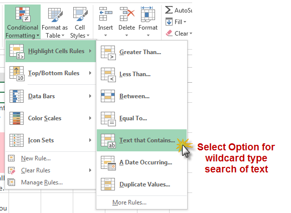
It could be troublesome if you have long list of comments and you want to highlight it for certain keywords like “good”, “bad”, “awesome” and so on. The Excel’s feature highlight containing text is the solution to this wildcard type search requirement. All you need is a cell dedicated for containing the criteria.

In this example, we will be examining the comments for an app from Google play store. Here are the comments:

We will setup first a cell that will contain our criteria – “annoying” for example. What we will do is to put these criteria in cell A1 and go to “Text that contain” text. The only thing we need to do is to point to the cell containing criteria. Once selected and pressed we are done.

Conclusion:

There are several ways we can format cells based on criteria in a cell. These were just few of them. Another option for formatting cell based cell values is to use VBA – but that is out of scope of this article. Please download the file from this link to see the formulas working.