Managing attendance of staff is a very critical issue, be it a manufacturing firm or a service firm. There are several tools out in the market to manage this function. This ranges from the simple spreadsheets to ERP system that is very complicated and are extremely reliable.
We at Excel zoom have produced a simple template to monitor the attendance of employees. This is a MS Excel based template that provided basic functionality to record attendance and analyses the basic features. So, let’s see how we can manage our firm’s attendance with this template.
The Template:
The Attendance template consists of three sheets:
- Data
- Summary_1
- Summary_2
Data
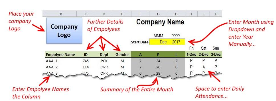
As the name suggests, this sheet is used to store data, for a month. You can enter the name of the of employees on the left most side and enter their details including the attendance on the right side onwards. On this sheet, we can set the month under consideration and the sheet’s date range will adjust automatically.
The sheet has date as header row and the date is adjusted automatically – using a formula and the options that the user enters in the cells marked for “Month” and “Year”. Once entered, the header row dates changes automatically.

In order to record the attendance, you can enter three options: A for absent, P for present and L for Leave, so that you can enter the appropriate option. The three columns besides the left most name column summarizes the employee’s performance by using formulas. You can see that summary of the attendance for the entire month is reported there.
The sheet has also provision to enter the ID of the employees that is essential to track them. Additionally the template has option to enter the department he is working in and the gender to further drill down the data. Following is the diagram showing the features.
Summary_1
This sheet provides further details and insights into the data you have collected through the daily attendance input. As you enter the data the sheet will be updated automatically.
This sheet uses the data from the “Data” sheet and provides absent percentage as percentage of total attendance. The next table to the right of this one is the sorted list of employees on the basis of highest percentage of absences. The table uses a complex formula (that will be described later sections of this article) to sort the list. Thus you can see who has highest number of absences in the office or which employee contributes highest to the total absences in the firm. You can use Pareto’s 80/20 rule to deal with such guys to reduce the number of absences.

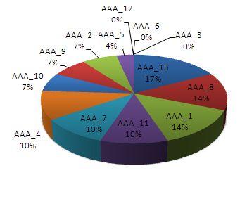
The third feature that is present in this sheet is a pie chart that shows distribution of absences over 360 degrees of circle. The chart is labeled for the data as well as the series names so that slices can be easily identified and makes understanding easier.

Summary_2
The third sheet shows the break up of attendance with respect to the departments. It is also important for companies to identify which department has most number of absences so that it can be advised to see the attendance issues – the sheets serves this purpose.
The sheet consists of department names in the left most column and the header row below which is reported the data. This data is again produced using a formula (and that will also be explained later in this article). The last column in the table reports the ratio of A+L over A+L+P so that you can see what the absence ratio for a particular department.

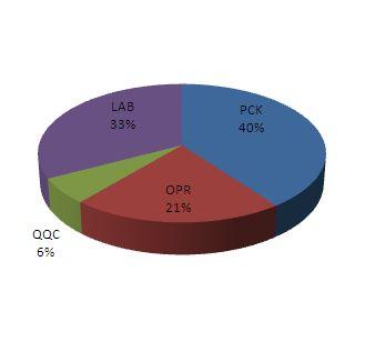
The second feature that can be used for analysis is again the pie chart on the right side. It simply shows the contribution of each department to make the 360 degrees of the pie. For our example, the highest chunk is occupied by PCK or packing department that reaches 40% of the total absences.
The footer row provides the column total and the overall ratio of absences for all the department is 7.97%.
So this was all about the template, in the next section we will se how to update the formulas in this template and try to understand the overall functions of the formulas used in this template.

Additional – Understanding the formulas
Formula No. 1
=SUMPRODUCT(($I7:$AM7=F$6)*1)
You will find this formula in cell F7 of “Data” sheet. Here I7:AM7 refers to the entire data table where we have been entering the attendance and F6 refers to the header row of the attendance summary table. As you drag the formula to the right, the referring changes to G6, H6 and gives the sum for all the three options (A, P, L). As such there is no need to change or update the formula because the template works for a month and there are no more then 31 days in month. If you want to make it for more then a month you need to change $AM7 to desired cell reference.
Formula No. 2
=DATE(H4,VLOOKUP($G$4,Sheet2!$B$3:$C$14,2,0),1)
This formula is present in the header row of the “Data” sheet in cell I6. The formula is responsible for providing the 1st date of every month by looking into a helper sheet (Sheet 2) and returning the month number. The month number is feed to the second argument of the DATE() function that return 1st date of any month you enter. This formula does not need to be updated unless you change the layout of your worksheet.
Formula No. 3
=IFERROR(IF(I6+1<=EOMONTH($I$6,0),I6+1,""),"")
This formula is found in the adjacent cells of I6 – from J7 onwards. This formula is used to truncate the month dynamically according to the number of days in the month. For example if Feb has 28 days, the attendance table will end at 28 and if May has 31 days, the table will go till 31st.
The formula check by checking if I6+1 IS less then the last date of the month that is found by using EOMONTH() formula. If the date is less, it will return the next day i.e. I6+1, other wise it will return blank cell. If there is an error, IFERROR() will return a blank cell.
Formula No. 4
=SUM(D4,F4)/SUM(D4:F4)+ROW(A1)/1000000
This formula is found in the Summary_1 in the cell G4 and downwards. The formula sums the A and L takes the ratio with A+L+P giving percentage absences. The second part of the formula with ROW() function adds and unique and very small number to the percentage to make it “unique” in case there are two cases with same percentage. This forms the basis of the sorted list in the next table.
Formula No. 5
=LARGE($G$4:$G$16,ROW(A1))
This formula finds the largest number of percentage based on the values in the last table. Since the values are made unique by adding very small number, the numbers are sorted easily.
Formula No. 6
=INDEX($B$4:$B$16,MATCH(J4,$G$4:$G$16,0))
This formula uses the percentage as matching criteria and then returns the corresponding employee name from the table. Since the lookup values are on the right side of the table, we can not use VLOOKUP() and hence INDEX() is used.
Formula No. 7
=SUMPRODUCT(($B4=Data!$D$7:$D$19)*(Summary_2!C$3=Summary_1!$D$3:$F$3)*(Summary_1!$D$4:$F$16))
This formula sums the parameters (A, P, L) on the basis of departments rather then employees. B4=Data!$D$7:$D$19 validates for the correct department, Summary_2!C$3=Summary_1!$D$3:$F$3 validates for the parameter i.e. A, P or L and the last portion represents the entire data table giving us the final count.
Conclusion:
So this is quite useful template from Excel zoom. Please use this link to download it and share your feedback in comments. Thank you.