Sometimes we get data in Excel that makes it somewhat difficult to look at the big picture. For example, you might get a list of transactions with a date and sale price. Let’s say you need to sum values in a month to use in some other analysis.
With that example, it isn’t easy to just look at the data and know that the first 10 rows are January’s transactions, the next 12 are February’s, etc. Analyzing the data could be even harder if all the transactions are out of order. However it isn’t terribly difficult to get a sum of values in a month.
Sum Values In A Month
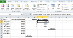
Let’s look at a simple example with two transactions per month for January, February, and March.
We are given the date of the transaction and the transaction amount but also want to find out the monthly totals. Now keep in mind that this is a simple example, but imagine if there were instead hundreds of transactions that need to be added up, the task could be much more difficult.

We will be using two formulas to get our answer: SUMPRODUCT and MONTH.
MONTH will produce a number between 1 (January) – 12 (December) given a particular date. For example, =MONTH(1/15/2014) will give a result of 1, because this date is in January.
SUMPRODUCT returns the sum of the products of a given range.
When we combine the two, we can use them to sum values in a month.
First set up your spreadsheet like in the screenshot above. Enter dates in A2:A7, dollar amounts in B2:B7, the numbers 1, 2, and 3 (for months January through March) in cells D2, D3, and D4 respectively. Finally, enter the following formula in cell E2:
=SUMPRODUCT((MONTH($A$2:$A$7)=D2)*($B$2:$B$7))
Then copy the formula down to E3 and E4.
Your spreadsheet should now have monthly totals for January, February, and March.
Obviously, in your actual worksheet you will replace the cell references with the applicable cells that you are working with. If you have a set of data that may encompass a variable number of rows (i.e. past row 7 in our example), you can replace $A$2:$A$7 and $B$2:$B$7 with A:A and B:B, which will use the entire column. However, please note that any errant text like a header row will cause an error in the formula.
You can also sum values in a year by replacing MONTH in the formula with YEAR, and replacing the numbers 1-3 in cells D2:D4 with years such as 2014, 2015, 2016, etc.