Introduction:
Just like other spreadsheet users, accountants do use a lot of formulas. It is not necessary that all the formulas that are used by accountant relate to their accounting functions. In order to make their sheets works and analyze data intelligently they use formula from across the categories provided in MS Excel: Lookup Function, Statistical Functions, Text Functions, Date & Time Functions and most importantly the Finance functions.
In this post we will take up ten functions that can be of real help to an accountant. As usual we will be explaining the use by referring to examples and in this post, we will try to explain by means of “Situational usage” of functions:
“What was the product cost for a Product in year 2014” – A case for VLOOKUP:
As the name suggests, the function is used for looking up values. For VLOOKUP to work, the data should be organized in a table, with header column containing the lookup value. The function provides option to select the column to look into and the type of match required.
For the case of looking up old product cost that is a common task for Accountant, we have to setup a table like below:

A VLOOKUP function set to do this job should look like:
=VLOOKUP(B9,$B$3:$E$7,4,0)
In this formula, the cell B9 refers to the lookup value, for our case we have Prod A as lookup value for first column. The second argument refers to the table range: $B$3:$E$7. The third option 4 is the fourth column in which we have to look into and the last option is for exact type match.
“What is the total investment made on buildings between 2010 and 2014” – An example use of SUMPRODUCT()
You may ask why SUMPRODUCT() and why not SUMIFS()? The answer lays in the layout of your sheet. If you want to answer the above question with SUMIFS() you must have your lookup data into columns i.e. years in columns. If you have your data in rows across the width of the sheet, you can’t use SUMIFS(). This is where SUMPRODUCT() shines, we can use it in either direction.
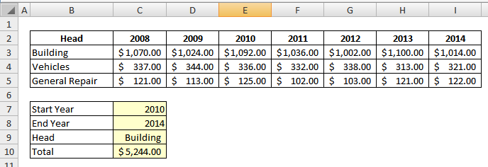
So lets consider the following table were various cost heads a reported for each year.

To get the result we will use the following SUMPRODUCT function:
=SUMPRODUCT((C2:I2>=C7)*(C2:I2<=C8)*(B3:B5=C9)*(C3:I5))
In this formula, the first argument (C2:I2>=C7) validates if the years in the row range are greater than or equal to the set value i.e. 2010. This is followed by another validation performed by (C2:I2<=C8) that checks if it is smaller than the end year. These two validations create a bucket-effect i.e. only years between this range will be considered in the formula.
The third part (B3:B5=C9) checks if the head is “Building”. All this result into a two dimensional array of 1 and 0 that is multiplied by range C3:I5. The result is then summed to give the final answer i.e. $5244.
“What was the total sales from Dallas in Feb 2017?” A possible use of SUBTOTAL() function.
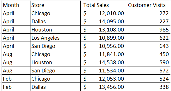
When data is organized is shape you list and you have to filter it for certain criteria, SUBSTOTAL is really a helpful function. It gives you a bunch of options to analyses the data and see results. Consider a case where a sales accountant has following data in hand and he has to answer question regarding sales performance:

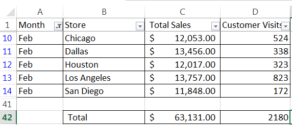
The question regarding sales for the month of Feb 2017 can be answered using filter feature the subtotal formula. We have written the formula in cell C42 and D42– keeping a row empty. When we filter the list for Feb 2017, we get this list as a result:

But this is for all the cities, filtering it down further we get…

The total sales from Dallas in Feb 2017 is 13456. And the total number of customer visits is 338.
The formula that we used here is SUBTOTAL(9,C2:C40) for total sales. The number 9 refers to the option “SUM” implying that the filtered data should be summed. The second option refers to the range that is going to be filtered.
Similarly in the next cell D42, we have used sum function again to get the count of total customer visits. A variation of this subtotal formula could be to use 1 for average, 4 for max and 5 for min functions.
“What has been the average head count for last 4 years?” An option to use AVERAGE() function.
A cost accountant keep track of the cost of human resource and workers. The function AVERAGE() can be of great help to them if they want to find averages, be it of head count of any other factor. Let’s consider the case where an accountant has successfully managed the record of head count for last 4 years and now management wants an overall average figure. Consider the following data to support our example:

The average head count for males can be found by averaging the first row and the count for females can be found by averaging for the second. And overall average can be found by using data in the last row.
The function we used here is =AVERAGE(C3:I3) where C3:I3 refers to the range containing data for male head count. The answer comes out to be 104.14
“What is NPV and IRR for this proposal?” – The way to NPV and IRR functions
Both functions are related to evaluating projects. NPV provides Net Present value and IRR gives internal rate of return. In order to find both we have to set up a sheet like below:

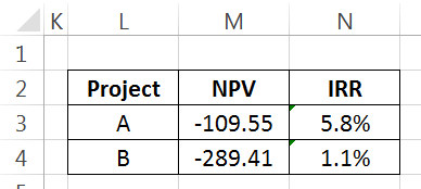
In this table, Rate is required for calculating NPV, where as for IRR we only need investment and outflows. When used formulas we have following output:

For calculating NPV in column M we have used following formula: =NPV(C3,D3:J3), in which C3 refers to the Rate (10%) and D3:J3 to inflow range. Similar for IRR the formula used is =IRR(D3:J3,0.1) in which D3:J3 is the same range and 0.1 represents an approximate guess for 10%.
Conclusion:
There are countless formulas with occasional and specific use. We have discussed jut few that we found useful for accountant. If you think any function should be added in this list, please mention it in comments. Please download the compassion file for this tutorial from this link.