Introduction to SUMPRODUCT:
In today’s post we will review some of the use of SUMPRODUCT function. The SUMPRODUCT function is amongst one of the favorites functions for Data Analysis – Particularly when you want to answer exploratory question like “how many”, “how frequent”, finding sum and averages against criteria’s. So we will start with a brief introduction of the SUMPRODUCTION function and in letter section will use example to explain the usage.
The Syntax:
The SUMPRODUCT function has only first argument as compulsory one, the rest of the arguments are optional. The function takes arrays of equal sizes that it multiplies and then returns the sum of the resulting array. The arrays must be of equal sizes otherwise the formula returns error. The function has following syntax.
SUMPRODUCT(array1, [array2], [array3], ...)
The syntax is adopted from MS help and we can see the only the first set of array is required, rest of them are optional (optional arguments are represented by square brackets). We can have up to 255 such arguments in SUMPRODUCT function.
Our Data
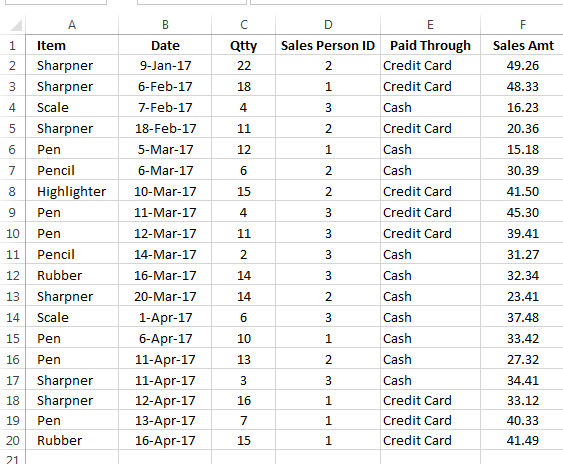
We have sample sales data for our analysis. The data has 6 fields namely Item, Date, Qtty, Sales Person ID, Paid through, Sales Amt. we will use this dataset to explain various uses of SUMPRODUCT.

EXAMPLES:
USING SUMPRODUCT TO SUM FOR AN ITEM:
Perhaps the simplest use of SUMPRODUCT is to sum a given range. For example referring to the above data, we can sum the quantity of pencil sold by using the following formula:
=SUMPRODUCT((A2:A20="Pencil")*(C2:C20))
This formula works by checking range A2:A20 for item pencil. Once found the corresponding value of quantity is multiplied with array of true and false, that is basically 1s and 0s and the final array is them summed to give total sales quantity for Pencil.
Tip: We can replace the fixed reference in the formula with a cell reference like one in the below example.
=SUMPRODUCT((A2:A20=H3)*(C2:C20))
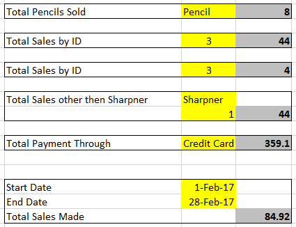
We can replace the value “Pencil” with cell reference H3.
USING SUMPRODUCT TO SUM FOR A CUSTOMER REPRESENTATIVE:
We have three customer representatives in the data identified by their IDs 1, 2 and 3. We can sum the total sales by using SUMPRODUCT again. The formula that will use is:
=SUMPRODUCT((D2:D20=H4)*(C2:C20))
In this formula, the first bracket is used to compare the customer representative ids with the one we want to sum sales quantity for. Thus we have comparison of an array of IDs with Customer ID = 3. The result is that multiplied with the respective values of sold quantity. The resulting array is then summed by SUMPRODUCT function.
USING SUMPRODUCT WITH OPERATORS FOR COMPARISON (GREATER THEN OPERATOR):
In Excel the operators used for comparisons used are following:

For example for finding no. of times sales was less than 3 for a customer representative could be done with following formula:
=SUMPRODUCT((D2:D20=H6)*(C2:C20<=4)*1)
The above formula first examines the range of IDs located in cell range D2:D20 and returns TRUE for cases where ID matches. This comparison is followed comparison of sales quantity with our criteria i.e. 4. This second comparison compares the quantity sold with the minimum set by user i.e. 4. Any sold quantity that is less than 4 will return a TRUE. These two arrays will be multiplied again to give yet another array of TRUE and FLASE – multiplying that array with 1 will then be summed up to have the final answer.
USING SUMPRODUCT WITH OPERATORS FOR COMPARISION (OTHER THEN OPERATOR):
We might want to count how many times a customer representative sold item other than pencil – in such case we will be using the “other than” operator (“<>”). For example if we want to find the sum of quantity of items sold by representative 1 other then sharpener then we can use following formula:
=SUMPRODUCT((A2:A20<>H8)*(D2:D20=1)*(C2:C20))
We can see that the formula uses other than operator in the first bracket. This operator makes sure that we have TRUE returned only for items other than our criteria – sharpener. The second comparison in the second bracket is confirms the correct ID of the representative and the product of these two arrays is multiplied with the quantity in the third array to give the result. In this example representative 1 has sold 44 items that are not sharpener.
USING SUMPRODUCT TO FIND THE PAYMENT THROUGH CASH OR CREDIT CARD:
A similar formula can be used find to find if payment has been made through credit card or in cash. For finding payments with SUMPRODUCT, we need to check the range containing payment option for these two payment methods.
The formula that will be used will be:
=SUMPRODUCT((E2:E20=H11)*(F2:F20))
In this formula the first bracket on the left evaluates if the value is equal to our choice – credit card, this returns an array of true and false and that is multiplied with the corresponding value of sales made. The resulting array is added up to give the answer.
USING SUMPRODUCT TO FIND THE SALES MADE IN A MONTH:
We can use DAY and MONTH function from excel to find the payment made in a certain month. Or alternatively we can set the start and the end date of the month to find sales in that particular month. Let’s assume that we want to set the start date of the month. We will calculate the end date with the help of formula.
Referring to the sheet the start date is present in cell I15, the next cell finds the ending date by making use of formula EOMONTH().
=EOMONTH(I15,0)
The next cell finds the total sales for a month (between start and the end date) with following formula:
=SUMPRODUCT((B2:B20>=I15)*(B2:B20<=I16)*(F2:F20))
The first bracket evaluates the date range for values greater then start of the month value, the second one evaluates the same range for dates that are less than or equal to the end date and then the resulting array of values is multiplied with total sales to give us the final answer.

CONCLUDING SUMPRODUCT:
There are still many more ways we can use SUMPRODUCT – please download the sample file to see how examples are setup.