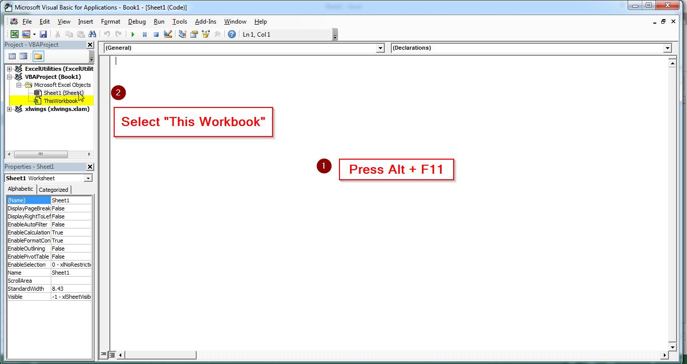
Archive

Archive for the ‘Macros’ Category

How to Recover Lost Excel Passwords
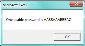
August 26th, 2009 2 comments

Let me preface this article by saying that this will not help you recover lost data, or gain access to protected data that you otherwise wouldn’t have access to.  What it will do is allow you to unlock a password protected worksheet in Excel, so that you can edit it as necessary.  Simply put, if you don’t already have access to the worksheet, this macro will not help you.

Now that the disclaimer is out of the way, let’s figure out why people password protect worksheets to begin with.  By protecting a worksheet and the contents of locked cells, users can keep themselves or other users from:

  • accidentally (or intentionally) removing formulas, or other contents of locked cells
  • adding or deleting rows and columns
  • changing cell, column or row formats
  • sorting data
  • using AutoFilter or PivotTable reports
  • editing objects or scenarios

Protecting a worksheet will not keep users from

  • editing any unlocked cells in the worksheet
  • viewing all data in the worksheet, regardless of if it is in a locked cell or not

Being able to unlock a password protected worksheet is useful, when

  • you have forgotten the password on your own worksheet
  • a co-worker, or other user has password protected a worksheet that you now need to edit, and they are not available to unlock the sheet for you
  • you have a need to perform an analysis of the data in a password protected worksheet, but are unable to do so due to the locked cells
  • you would like to sort/filter the data in a password protected worksheet, or create a PivotTable report from the data

Since Microsoft Excel is not a “secure” program, it is very easy to unlock the password of a password protected worksheet.  This is because there are several different combinations of passwords that Excel will accept to unlock the worksheet.  For example, a worksheet with the password “treehouse”, can also be unlocked with the password “AAAABAABBBB/”.  The opposite is also true (i.e. protecting with the password “AAAABAABBBB/” can be unlocked with the password “treehouse”).  Go ahead; try locking a worksheet with the password treehouse, and use AAAABAABBBB/ to unlock it.

The macro code below will “unlock” one worksheet at a time, using the method used above.  It won’t provide you with the actual password someone typed in, but rather a random sequence of letters or symbols that will work to unlock the worksheet.


Sub PasswordRecovery()
'
'MACROS BY EXCELZOOM.COM
Dim i As Integer, j As Integer, k As Integer
Dim l As Integer, m As Integer, n As Integer
Dim i1 As Integer, i2 As Integer, i3 As Integer
Dim i4 As Integer, i5 As Integer, i6 As Integer
On Error Resume Next
For i = 65 To 66: For j = 65 To 66: For k = 65 To 66
For l = 65 To 66: For m = 65 To 66: For i1 = 65 To 66
For i2 = 65 To 66: For i3 = 65 To 66: For i4 = 65 To 66
For i5 = 65 To 66: For i6 = 65 To 66: For n = 32 To 126
ActiveSheet.Unprotect Chr(i) & Chr(j) & Chr(k) & _
Chr(l) & Chr(m) & Chr(i1) & Chr(i2) & Chr(i3) & _
Chr(i4) & Chr(i5) & Chr(i6) & Chr(n)
If ActiveSheet.ProtectContents = False Then
MsgBox "One usable password is " & Chr(i) & Chr(j) & _
Chr(k) & Chr(l) & Chr(m) & Chr(i1) & Chr(i2) & _
Chr(i3) & Chr(i4) & Chr(i5) & Chr(i6) & Chr(n)
Exit Sub
End If
Next: Next: Next: Next: Next: Next
End Sub

Categories: Macros Tags: , , ,

Confirmation Before Execution

May 9th, 2009 1 comment

Often times when you execute a macro, the process isn’t easily undone. You may have a macro that deletes certain information, or completely reformats your worksheet. In either case, you want to be sure that your workbook’s users are absolutely certain that they are ready to execute the macro before running it. If the macro can be run by clicking on an object within the worksheet, an accidental click may cause unintended consequences.

The code below will produce a pop up box as soon as the macro is run. It will ask the user if they are certain that they want to run the macro, and give them the option to proceed, or cancel it right there. Think of it like when you’re about to delete a file from your computer and Windows asks “Are you sure you want to move this file to the Recycle Bin?”. Clicking “Yes” will delete the file, and “No” will cancel the process.

You can edit the text to be displayed in between the quotes “Do you want to run this macro?”. The code will produce two options “OK” and “Cancel”. If you want it to produce “Yes” and “No”, change the vbOKCancel to vbYesNo, and vbCancel to vbNo. Both will do the same thing, it just depends on how you want to present the question.

Copy all the code below. Paste it into your workbook’s Visual Basic editor, either under a Microsoft Excel Object or Module. Replace ** YOUR MACRO CODE HERE ** with your macro’s commands.

Need help? Use our nifty guide to help figure out how to install and use your macros.

Sub Confirm_Macro()
'
'MACROS BY EXCELZOOM.COM
'
If MsgBox("Do you want to run this macro?", vbOKCancel + vbQuestion) = vbCancel Then
Exit Sub
Else
** YOUR MACRO CODE HERE **
End If
End Sub

Categories: Macros Tags:

Hide/Unhide Columns

April 25th, 2009 No comments

On occasion, you might find yourself creating a spreadsheet that has multiple columns all set up in a consistent format (i.e. quarterly sales figures for the past 5 years). As time goes on, you may add/remove data to the spreadsheet as needed. This may result in some columns not being used (i.e. in April only the first quarter’s information will be filled out for the current year, leaving the second, third and fourth quarters blank).

Excel Hide Column Macro

Using the quarterly sales example above, assume that you’ve taken the time to set up your spreadsheet with placeholder columns for the remainder of the year. When printing the information, you don’t want to just delete the columns, only having to recreate them in the future, and you also don’t want to have to manually hide/unhide them either.

You can use a macro to toggle between hiding and unhiding these empty columns fairly easily. The first bit of code will determine if the total in row 8 for columns B through M is 0. If it is, it will hide the column, otherwise it will make sure the column is not hidden. The second bit of code will select columns B through M and make sure they all are not hidden, so that you can toggle between hiding the unused columns, and showing all the columns.

To use this in your own spreadsheet, you may need to change a few things. 1) Change the Range reference (i.e. “B8:M8″) to whatever range you want evaluated. 2) Change “Columns” in Rng = Selection.Columns.Count to “Rows” if the range you are evaluating is a range of rows not columns. 3) If the criteria is something other than “0″, change the “0″ in If ActiveCell = 0 to whatever that criteria happens to be. And finally 4) the two lines that say ActiveCell.Offset(0, 1).Select simply moves the selected cell down 0 cells and to the right one cell. If you’re evaluating down a range of rows, change the 0 to a 1 and the 1 to a 0 so that it moves the selected cell down 1 cell and to the right 0 cells. (Note you can move up a cell by inserting a -1 as the first number and to the left by inserting a -1 as the second number).

Need help? Use our nifty guide to help figure out how to install and use your macros.

Hide Unused Columns:

Sub hide_unused()
'
'MACROS BY EXCELZOOM.COM
'
Application.ScreenUpdating = False
Range("B8:M8").Select
Rng = Selection.Columns.Count
For i = 1 To Rng
If ActiveCell = 0 Then
Selection.EntireColumn.Hidden = True
ActiveCell.Offset(0, 1).Select
Else: Selection.EntireColumn.Hidden = False
ActiveCell.Offset(0, 1).Select
End If
Next i
Application.ScreenUpdating = True
End Sub

Unhide all Columns:

Sub unhide_all()
'
'MACROS BY EXCELZOOM.COM
'
Application.ScreenUpdating = False
Columns("B:M").Select
Selection.EntireColumn.Hidden = False
Application.ScreenUpdating = True
End Sub

Categories: Macros Tags: , ,

Using a For Loop

April 11th, 2009 No comments

 ”For” loop is used in a macro whenever you have an action that needs to be performed a set number of times. For example, if you want to change the fill color of the first 20 cells in a list, you could have the macro select the range and simply fill as desired. But what if you wanted to only fill the cells if they were blank, for example? Telling the macro to select the whole range and fill it wouldn’t work.

This is where a “For” loop is useful. You can have the macro to go down your list, and determine if the cell is blank. If it is, then have the macro fill the cell with a color, otherwise go to the next cell, until it has run through the whole list.

The following code will do exactly what was mentioned above.

Sub FLoop()
'MACROS BY EXCELZOOM.COM
For x = 1 To 20
Cells(x, 1).Select
If Selection.Value = "" Then
With Selection.Interior
.Color = 65535
End With
End If
Next x
End Sub

  • The first line identifies the range of rows to be evaluated. It also tells the macro, that if ‘x’ is less than 20, keep on going.
  • The next line tells the macro to select the cell in column 1.
  • The ‘If’ section determines if the selected cell is blank, and if it is, it will fill it with a color (in this case 65535=yellow), and if it isn’t blank then just move on and evaluate the rest of the cells until the end of the range.
Categories: Macros, Tips Tags: ,

Automatically Create an Index for Your Excel File

March 12th, 2009 No comments

Do you want one central location where you can easily navigate to any worksheet in your file, and then navigate back with one click? This macro creates an index that lists all sheets in your workbook. The best part is that the index excel macro updates itself everytime you select the index sheet.

If you need an index sheet in your file, you probably already have a zillion worksheets in your file, but add one more, and call it “Index”, or whatever you want to identify it as an index (table of contents, etc.). Next, right click the Index tab and select ‘View Code’. This is where you will enter the code below. Click on another sheet in your file, then click back on your Index sheet. You’ll notice that it has populated a list of all the sheets in your file, complete with a convenient link to them. In all your other sheets, cell A1 will have a “Back to Index” link for easy navigation. If you want to use another cell for this backwards navigation, change the code in both places where it says A1 to whatever cell you’d like.

Need help? Use our nifty guide to help figure out how to install and use your macros.


Private Sub Worksheet_Activate()
'
'MACROS BY EXCELZOOM.COM
'
Dim wSheet As Worksheet

Dim l As Long

l = 1

With Me

.Columns(1).ClearContents

.Cells(1, 1) = "INDEX"

.Cells(1, 1).Name = "Index"

End With

For Each wSheet In Worksheets

If wSheet.Name <> Me.Name Then

l = l + 1

With wSheet

.Range("A1").Name = "Start_" & wSheet.Index
.Hyperlinks.Add Anchor:=.Range("A1"), Address:="", _
SubAddress:="Index", TextToDisplay:="Back to Index"

End With

Me.Hyperlinks.Add Anchor:=Me.Cells(l, 1), Address:="", _
SubAddress:="Start_" & wSheet.Index, TextToDisplay:=wSheet.Name

End If

Next wSheet


End Sub

Categories: Macros Tags:

Send Emails From Excel

March 4th, 2009 No comments

Often times you’ll find yourself working on a file in Excel that needs to be sent to a co-worker as an attachment. If you store your files on a shared network drive, it could take a little while to find your file, even if you know exactly where it is located. Even then, you may have to worry about attaching the wrong file if there are several saved with similar file names.

By using the macro below, you’ll be able to attach the file you have open to an email with the click of a button.

Copy all the code below. Paste it into your PERSONAL.XLS workbook’s Visual Basic editor, under a Module. The following steps also need to be completed to use this macro:

  • Change “someone@example.com” to the email address of the person you want to send your file to
  • The line “This Email was sent on ” & Format(Date, “mmmm dd, yyyy”) is the subject line. Change it to whatever you would like your subject to say. This one would read “This Email was sent on March 04, 2009″ assuming today was March 04, 2009.

Need help? Use our nifty guide to help figure out how to install and use your macros.

Sub email_active_workbook()
'
'MACROS BY EXCELZOOM.COM
ActiveWorkbook.SendMail "someone@example.com", _
"This Email was sent on " & Format(Date, "mmmm dd, yyyy")
End Sub

Categories: Macros Tags: ,

Create and Name a New Worksheet

March 1st, 2009 No comments

Say you have a spreadsheet that keeps track of weekly sales information, which you want displayed in a new sheet for each month. You don’t want to copy an “original” worksheet each week, so a macro can help to automate this process.

The macro code below will copy the worksheet named “Original”, and place it after the last worksheet in your file. It will then prompt you to enter in the date that corresponds with that week. It will continue to do so until you enter a valid worksheet name (i.e. valid format and a name that isn’t already used somewhere else in the workbook. Make sure your workbook already has a file called “Original”, and it is formatted the way you want all your weekly reports to be formatted. (Note if your “Original” worksheet isn’t called “Original”, you can change the name in the macro code below to whatever you want).

Copy all the code below. Paste it into your workbook’s Visual Basic editor, either under a Microsoft Excel Object or Module.

Need help? Use our nifty guide to help figure out how to install and use your macros.

Sub CopyNewSheet()
'
'MACROS BY EXCELZOOM.COM
'
Dim shname As String
Dim wrksh As Worksheet
Worksheets("Original").Copy after:=Sheets(Worksheets.Count)
Set wrksh = ActiveSheet
Do While shname <> wrksh.Name
shname = Application.InputBox _
(Prompt:="Enter This Week's Date")
On Error Resume Next
wrksh.Name = shname
On Error GoTo 0
Loop
Set wrksh = Nothing
End Sub

Categories: Macros Tags: ,

Format a List in Columns to a Single Column

February 21st, 2009 No comments

Say you have a large contact list in Excel that is formatted, for example like: Column A – Names, Column B – Addresses, Column C – Cities, Column D – States, Column E – Zip Codes. It’s great that everything is formatted in neat columns, but it would be a nightmare if you wanted to use this list to print off envelope address lables.

Thankfully, there’s a macro can speed up this process. The macro below assumes that you’re starting in the left most column in your list (in my example, column A), and will insert three rows below (one for the address, one for the city, state and zip, and one blank one between records). It then takes the address from the second column (column B) and puts it below the name (row 2). It then proceeds to take the city, state and zip and puts them in the appropriate columns below the address (in row 3). Finally, it will move down to row 5, where the next record starts and repeats the process over again. It will continue to repeat (or loop) until it runs into a blank cell in column A. The result is a list of all your contacts formatted to be used on an envelope.

You’ll also notice that I added “Application.ScreenUpdating = False” to keep the screen from updating everytime the macro did something. If you have a list with a few hundred or even thousands of people it would get pretty obnoxious to see the screen flicker everytime something was cut and pasted. At the end “Application.ScreenUpdating = True” is added to allow Excel to reveal the final masterpiece.

I only wish I thought of this macro when I was formatting my wedding invitation list!

Copy all the code below. Paste it into your workbook’s Visual Basic editor, either under a Microsoft Excel Object or Module.

Need help? Use our nifty guide to help figure out how to install and use your macros.

Sub FormatList()
'
'MACROS BY EXCELZOOM.COM
'
Application.ScreenUpdating = False
Do Until ActiveCell.Value = ""
ActiveCell.Offset(1, 0).Range("A1:A3").Select
Selection.EntireRow.Insert
ActiveCell.Offset(-1, 1).Range("A1").Select
Selection.Cut
ActiveCell.Offset(1, -1).Range("A1").Select
ActiveSheet.Paste
ActiveCell.Offset(-1, 2).Range("A1").Select
Selection.Cut
ActiveCell.Offset(2, -2).Range("A1").Select
ActiveSheet.Paste
ActiveCell.Offset(-2, 3).Range("A1").Select
Selection.Cut
ActiveCell.Offset(2, -2).Range("A1").Select
ActiveSheet.Paste
ActiveCell.Offset(-2, 3).Range("A1").Select
Selection.Cut
ActiveCell.Offset(2, -2).Range("A1").Select
ActiveSheet.Paste
ActiveCell.Offset(2, -2).Range("A1").Select
Loop
Application.ScreenUpdating = True
End Sub

Categories: Macros Tags: ,

Run Macro At a Specified Time

February 18th, 2009 No comments

Using the Application.OnTime Method will allow you to schedule a macro to be run at a specified time. The specified time can be either after certain amount of time has passed, or at a certain time of day. This is especially useful if you would like a daily or weekly report to be printed, without having to be around to print it. If the report is long, it might take a while to print, so it might be useful for the macro to run after business hours or on the weekend.

The only drawback to this macro is that the file must be open in order for it to run. You can have this automated for you by using the Windows Scheduler found in the Control Panel to open the file at a certain time, and have the code below run automatically when opened.

Copy all the code below. Paste it into your workbook’s Visual Basic editor, in a Module. Replace “my_macro” with whatever name you have given your macro.

Need help? Use our nifty guide to help figure out how to install and use your macros.

The code below will allow you to run a macro called “my_macro” 30 seconds from now. You can change the time to whatever time interval you would like.

Sub Run_After_30_Sec()
'
'MACROS BY EXCELZOOM.COM
'
Application.OnTime Now + TimeValue("00:00:30"), "my_macro"
End Sub

Use the following if you wish to run the macro at a certain time of day. The code below will automatically run my_macro at 5pm (written in 24 hour time as 17:00:00).

Sub Run_At_5PM()
'
'MACROS BY EXCELZOOM.COM
'
Application.OnTime TimeValue("17:00:00"), "my_macro"
End Sub

Categories: Macros Tags: ,

Change Text Case to lower, UPPER, or Title Case

February 11th, 2009 No comments

Do you want to have a list of information in all CAPITAL LETTERS, all lower case, or All In A Title Format? This would be an extremely tedious task if, say you have 100+ lines that need to be updated. With these macros, you can select the cells you wish to update and change their case in a flash!

Note: These macros won’t change the output of a cell with a formula in it.

Copy all of the code below. Paste it into your workbook’s Visual Basic editor, either under a Microsoft Excel Object or Module.
Need help? Use our nifty guide to help figure out how to install and use your macros.

Lower Case:

Sub TextLowerCase()
'
'MACROS BY EXCELZOOM.COM
'
Dim cell As Range
For Each cell In Selection.Cells
If cell.HasFormula = False Then
cell = LCase(cell)
End If
Next
End Sub

Upper Case:

Sub TextUpperCase()
'
'MACROS BY EXCELZOOM.COM
'
Dim cell As Range
For Each cell In Selection.Cells
If cell.HasFormula = False Then
cell = UCase(cell)
End If
Next
End Sub

Title (Proper) Case:

Sub TextTitleCase()
'
'MACROS BY EXCELZOOM.COM
'
Dim cell As Range
For Each cell In Selection.Cells
If cell.HasFormula = False Then
cell = Application.Proper(cell)
End If
Next
End Sub

Categories: Macros Tags: ,