Excel Tip #4: Filter Your Data
If you are working with a spreadsheet with a large set of data, you may be able to speed up your work by filtering the data to only display the information you are concerned with at the moment.
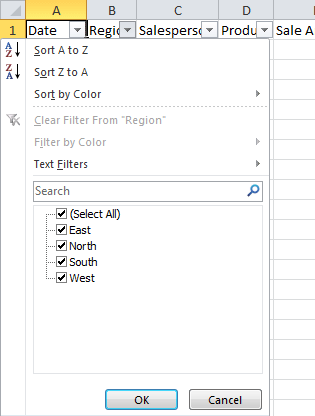
For example, if you have a spreadsheet with sales data for your company across all the regions it operates in, you can filter the data by region to show only that region’s results.
To filter your data:
- Click the cell in the top left of your data set.
- Click the Data tab, then the Filter button in the Sort & Filter group.
- There should be some arrows like a drop-down menu in each of the cells in the top row.
- Click on the arrow in the column you want to filter by.
- Place a check mark next to each data group you are interested in.
- Click OK.
- You can filter by more than one column, so if you want to only see the sales from the East region in May, you can filter by both the Region and Date columns.
- Your data will now only show the data you want to see.
- To see all data again, click the arrow button again, and click the Select All option.
